Wide-Table Denormalization Tradeoffs in OLAP
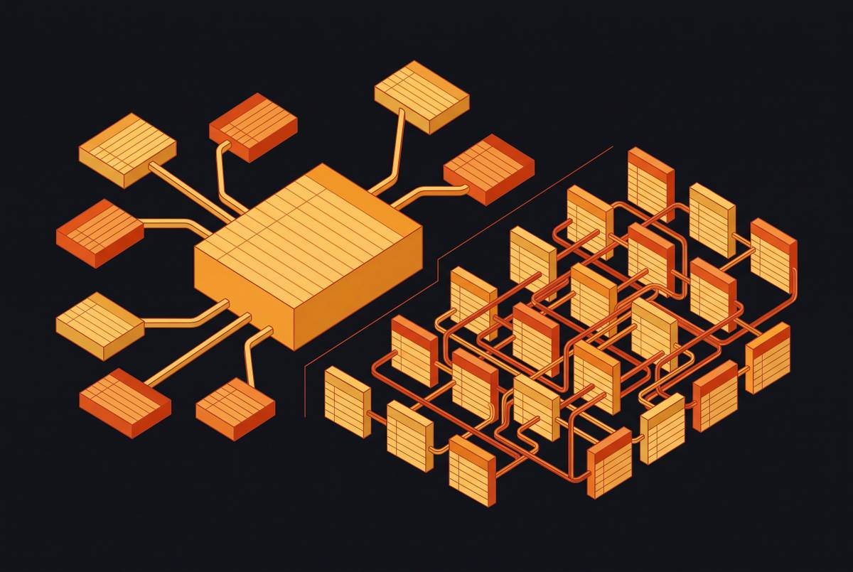
Columnar storage changed join economics but did not eliminate the denormalization tradeoff.
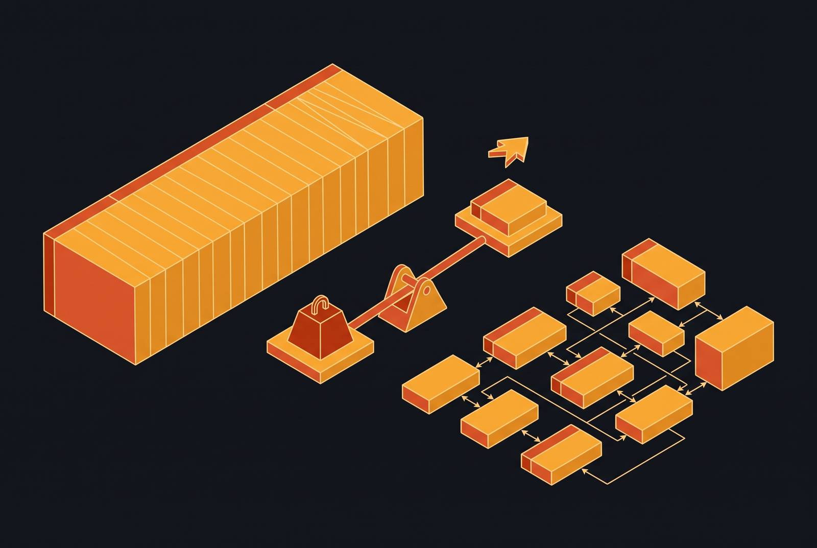
OLAP engines once forced a choice: normalize the schema and live with slow joins, or flatten everything and live with painful updates. Columnar storage and vectorized execution changed the arithmetic, but they didn't remove the tradeoff. They moved it. Understanding which problem you actually have is the prerequisite for every schema decision that follows.
Why OLAP engines changed the join calculus but did not eliminate the tradeoff
Older analytical databases struggled with multi-table joins under concurrency, and so denormalization became the default. Response times ranged from sub-second to minutes, and sub-second was not the standard SLA target. Flattening was the obvious path because the alternative was visibly slower.
That calculus has shifted. Some modern OLAP engines now handle star schemas and complex cross-table joins at scale. Others, like Apache Druid and Pinot, still require denormalization for most join workloads. Teams now face a real architectural choice rather than a foregone conclusion. Flattening is no longer the only path to query performance, and the choice carries consequences in both directions.
What columnar storage actually neutralizes and what it does not
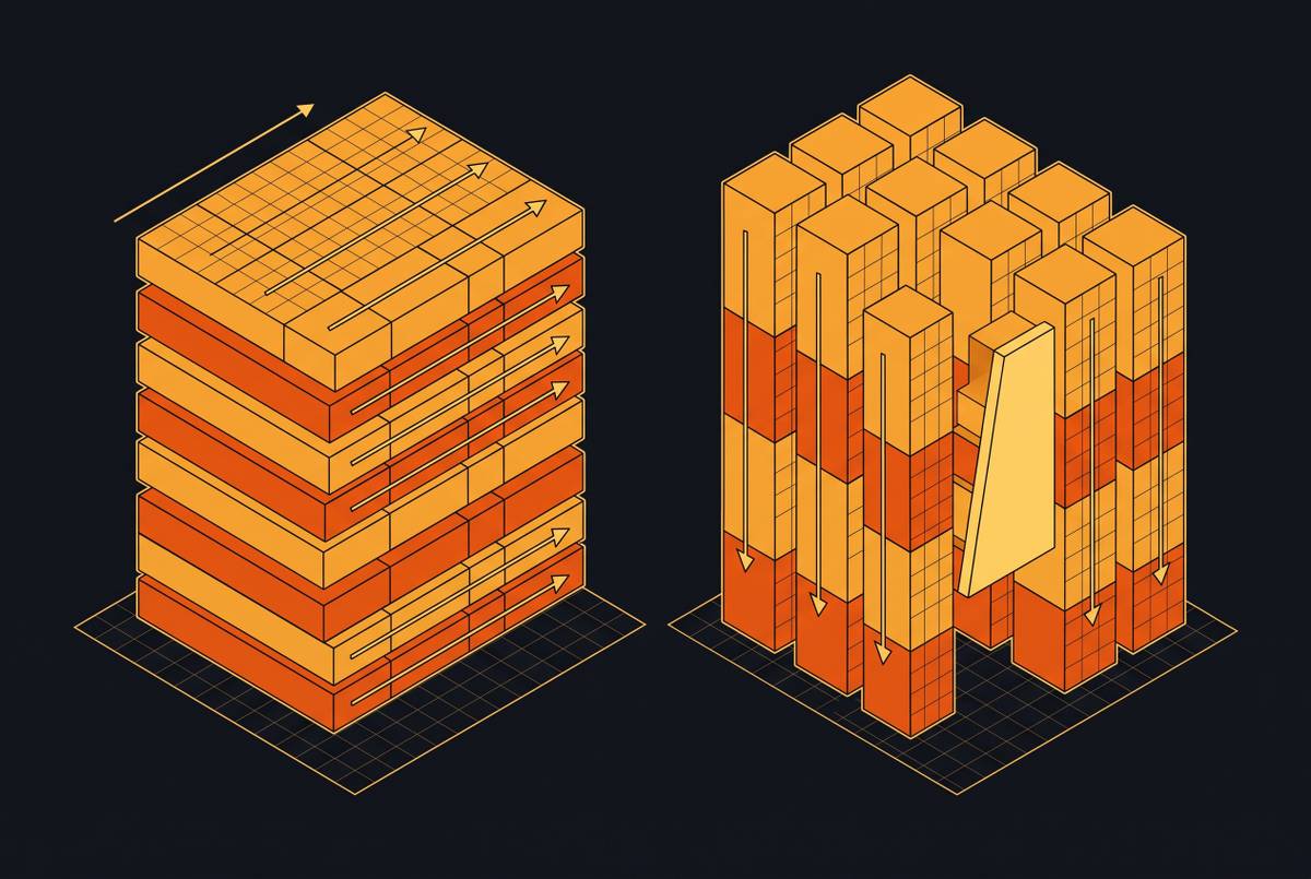
Columnar storage neutralizes the scan penalty of extra columns but leaves write amplification, update complexity, and storage cost fully intact. Distinguishing these is the foundation of any honest denormalization decision. What columnar storage genuinely eliminates is the row-store penalty. A row-store engine reads entire rows, no matter which columns a query touches. A columnar engine skips columns not in the query entirely. A filter on date, state, and total_amount is not affected by the existence of a category column. The engine never reads that column segment. Vectorized execution compounds this benefit: once the engine locates the right column segment, SIMD instructions process large batches of values per CPU tick. If you pre-join dimension attributes into a fact table, the query can skip the join. The query accesses one column segment instead of coordinating two. Reduced join depth also improves caching efficiency for aggregation-heavy analytical queries, and denormalized structures can better support indexing strategies and pre-aggregated summary tables.
What columnar storage does not touch is the write side. Embedding a customer's city in every order row means updating many rows when that city changes, not one row in a customers table. Update anomalies are inherent to denormalization regardless of the read engine. Storage cost also persists: duplicate fields occupy real space, and a denormalized table can be substantially larger than the normalized equivalent. That larger footprint evicts more pages from the buffer pool, and in cloud warehouses larger scan targets can raise on-demand query costs. Dictionary encoding limits but does not eliminate storage growth. It offsets overhead, not all of it.
A separate failure mode emerges at extreme column counts. Memory spikes and file-open latency represent a qualitative change in behavior, not just gradual degradation. The performance curve is not linear.
The costs that actually dominate: write amplification, update complexity, and grain mixing
The practical risks of aggressive denormalization are not scan performance or storage size. They are the three problems that emerge at write time and schema-design time: update anomalies, pipeline complexity, and grain mixing. Update anomalies are the most concrete operational risk. Denormalization trades storage efficiency for query speed, and the write side of that trade is non-trivial. Every row that carries a redundant field must keep it consistent. High-frequency transactional writes make this expensive. Updating a customer attribute in a denormalized table means touching many rows, not one. Schema evolution becomes structurally harder too. Adding a new data source or changing a field definition can require rebuilding the entire wide table. Slowly-changing dimensions are handled naturally by a normalized model and awkwardly by a wide table.
Pipeline complexity is the hidden cost. Keeping redundant data consistent requires disciplined ETL or CDC pipelines. If those pipelines fail, inconsistency appears in query results without obvious signals. Redundancy across datasets complicates version control for multiple downstream pipelines that all read from the same wide table. The governance cost is often invisible at build time. A star schema forces the analyst to choose the join and therefore the semantics. A wide table bakes that choice in silently, and readers months later were not in the room when it was made.
Grain mixing is the worst wide-table failure mode in production. Wide tables do not resist mixed grains by design. The schema permits header attributes to fan out across line rows, and aggregates to sit beside the details they aggregate. An order-header field duplicated onto every line-item row is the classic case. This produces query results that are correct by type but wrong by semantics. That category of error is harder to detect than a runtime failure.
When flattening is the right call: query patterns that justify a wide table
Denormalization is justified when the query pattern is stable, the write frequency is low relative to read frequency, and the join depth in the normalized model demonstrably creates latency. Not before all three conditions are met. The read-to-write ratio is the primary signal. The rule is to normalize until joins hurt, then denormalize until they work, then stop. Denormalize only when a production query proves the join cost exceeds insertion-time replication cost. Read-heavy, write-light patterns are the canonical case where the tradeoff favors flattening. The data loads once through batch ETL or low-frequency CDC, and is queried many times. The replication cost is paid once. The join savings accrue on every query.
Specific workload types favor wide tables. Dashboard and reporting workloads with stable, recurring query patterns over large row counts are the clearest fit. Pre-computed summary tables for monthly or daily aggregations carry all needed columns with no join at query time. Flatten real-time analytics for customer-facing products when p99 latency is a product requirement, not a preference. In these cases the write pipeline is owned and controlled, and update anomalies are a known cost the team has chosen to manage. Self-service BI environments also benefit: business users selecting fields in a BI tool get better results from a wide, flat table than from a join graph they do not understand.
Workloads where denormalization is the wrong tool deserve equal clarity. High-frequency transactional writes make redundancy expensive to maintain. Financial and audit systems need strict consistency. Small datasets have negligible join cost, and premature denormalization doubles write amplification and creates data-integrity bugs without a meaningful performance return.
The hybrid patterns that avoid the binary choice
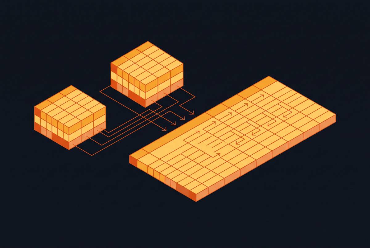
The most durable production pattern is not full normalization or full denormalization but a hybrid. Keep writes normalized, and materialize wide tables only for the read paths that need them. CDC is the canonical bridge between OLTP normalization and OLAP denormalization. Normalized OLTP in PostgreSQL or MySQL replicates through change-data-capture into an OLAP engine for denormalization. OLTP stays fast with small, normalized writes. Analytics gets the wide tables it needs. Log-based CDC tools like Debezium and Streamkap can move OLTP changes into OLAP stores in single-digit seconds. Managed ELT platforms that use CDC typically deliver changes in minutes. That enables near-real-time freshness without sacrificing OLTP write performance. This pattern separates the update-anomaly problem from the query-performance problem. Each side is solved in its appropriate system.
Materialized views offer targeted denormalization without changing the underlying schema. Precomputing and storing the results of complex joins or aggregations speeds up reads for data patterns you access often. The materialized view is rebuilt or incrementally updated on a schedule. The base tables remain normalized and consistent. This pattern directly addresses the governance problem: the join semantics are defined once in the view definition, versioned, and reusable, not re-derived independently by each analyst.
Virtual denormalization through SQL views is a lower-commitment option. A view joins and flattens normalized tables into a single logical surface. Consumers query it as if it were one wide table, but the underlying data remains normalized. The tradeoff is that views execute joins at query time, which can be slow for very large datasets. Materialization closes that gap when latency requires it. The discipline is to define join logic once in the view, version it, and let all consumers use the same definition. That prevents semantic drift across teams.
Calculated and pre-aggregated columns are a scoped form of denormalization. Storing derived values like net_revenue (calculated as quantity multiplied by unit_price multiplied by one minus discount) alongside raw data eliminates repeated in-query computation without requiring full table flattening. This is denormalization at the column level, not the table level. It is a narrower commitment with proportionally narrower maintenance cost.
How wide tables change what AI agents can reliably do with your schema
Schema design for OLAP is no longer purely a human-analyst concern. AI agents querying a warehouse generate SQL from schema structure. Wide tables reduce the combinatorial surface where agents produce incorrect queries, but only up to the point where column semantics are explicit.
Agents generate more accurate SQL against wide, flat schemas for a straightforward reason. Fewer joins and simpler schema structure reduce the surface where an agent can generate an incorrect join condition or hallucinate a relationship between tables. An agent that writes SQL against a wide table with all relevant columns in one place has fewer opportunities for a structurally valid but semantically wrong query. You can see the reasoning: each join is a decision point, and each decision point is a place where the agent can get lost.
The limit of schema simplicity arrives quickly. Raw event tables carry no inherent business meaning. Concepts like activation or churn must be explicitly defined. A flat schema that does not encode those definitions does not help an agent more than a normalized one. A semantic layer mapping human concepts to schema elements is the prerequisite for reliable AI analytics. A wide table without it still produces wrong answers, just through a different failure mode. Enterprise NL-to-SQL accuracy drops sharply when questions involve multi-step business logic, ambiguous column semantics, or cross-table joins. Schema shape alone does not solve this.
The access layer needs more than schema design. Agents that probe data relentlessly and in parallel create a different query pattern from human analysts: high concurrency, iterative sub-questions, automated drilling. That pattern demands isolation and auditability, not just a flat schema. Isolated, read-only compute for agent workloads prevents an agent's exploratory queries from contending with production analytical traffic. Full query logging is required for agentic access to remain accountable. Autonomous does not mean unaccountable, and every agent query against a production dataset should be recoverable for review. Sandboxed branches that let agents experiment against real data without touching production reduce the risk surface. Structured schema tooling extends the denormalization decision too. When agents interact with schema as code, a well-structured wide table with explicit column semantics is more amenable to agent-driven schema operations than an ad-hoc flat table assembled for convenience.
A decision framework for when to denormalize, when to stop, and what to monitor afterward
The denormalization decision reduces to three sequential questions. Does the measured query pattern actually require it? Can the update complexity be managed by the team's pipeline discipline? Does the monitoring layer catch consistency drift before users do?
Start by measuring before flattening. Normalize by default. Denormalize only when a production query proves the join cost exceeds insertion-time replication cost. Identify the most-queried reports or dashboards, and count the joins in the underlying SQL. If the join count is high and query latency fails the SLA, that is the signal to consider flattening that specific path. Small datasets, infrequent queries, or queries that already meet latency targets do not justify denormalization. The redundancy cost is real, and the performance return is negligible.
Then choose the lightest commitment that solves the problem. Calculated columns denormalize at the column level for derived values before you flatten entire tables. Materialized views physically materialize specific join paths on a schedule while keeping base tables normalized. That is the right level for most BI workloads. Full wide-table flattening is justified when write frequency is genuinely low relative to read frequency, update anomalies are manageable, and the query pattern is stable enough to make rebuilding the table rare. The workload decision matrix maps the choice: read-heavy and write-light with a stable query pattern makes full denormalization defensible; read-heavy and write-light with an evolving query pattern favors materialized views; mixed read/write calls for a hybrid with a normalized core and a denormalized read layer via CDC; write-heavy or strict-consistency workloads should stay normalized because denormalization creates more problems than it solves.
Managing grain and semantics is a design-time discipline, not an afterthought. Define the unit of a row explicitly and enforce it. Do not let header attributes fan out across line-item rows for convenience. Encode business semantics in the schema or view definition, not in individual queries. That is the prerequisite for both reliable analyst queries and reliable agent-generated SQL.
Finally, monitor for the failures denormalization introduces. Schema tracking watches table structure and detects changes like added or removed columns and datatype modifications, catching structural drift before BI users hit it. Timeliness monitoring detects missing data arrivals. A wide table built from a CDC pipeline that silently stops propagating updates is a consistency failure, not a schema failure. Validation runs business rule checks that catch anomalies in redundant fields. If the same customer city appears in two different values across rows that should agree, the pipeline has drifted. Different observability tools address different risks, and all three matter.
Denormalization is not a one-time schema decision. It is an ongoing operational commitment. The engine gives you room to choose, but the write paths, the pipeline discipline, and the monitoring layer determine whether the choice holds up.