Percentile Reporting Standards for Database Latency Benchmarks

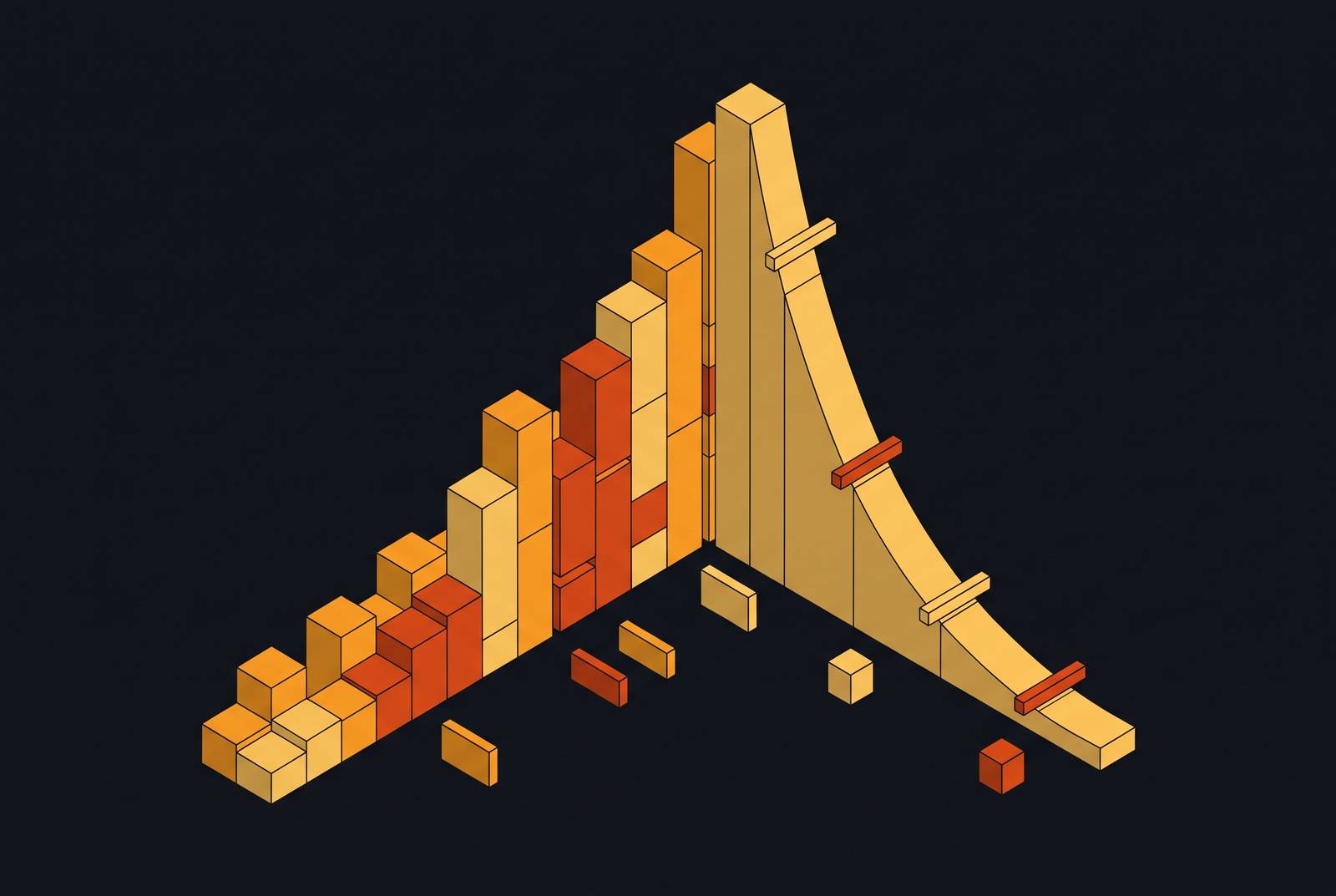
A single average can't tell you what a latency distribution actually looks like, because latency almost never distributes evenly. It skews right, hard, with a long thin tail of slow requests dragging the mean away from what nearly everyone experienced.

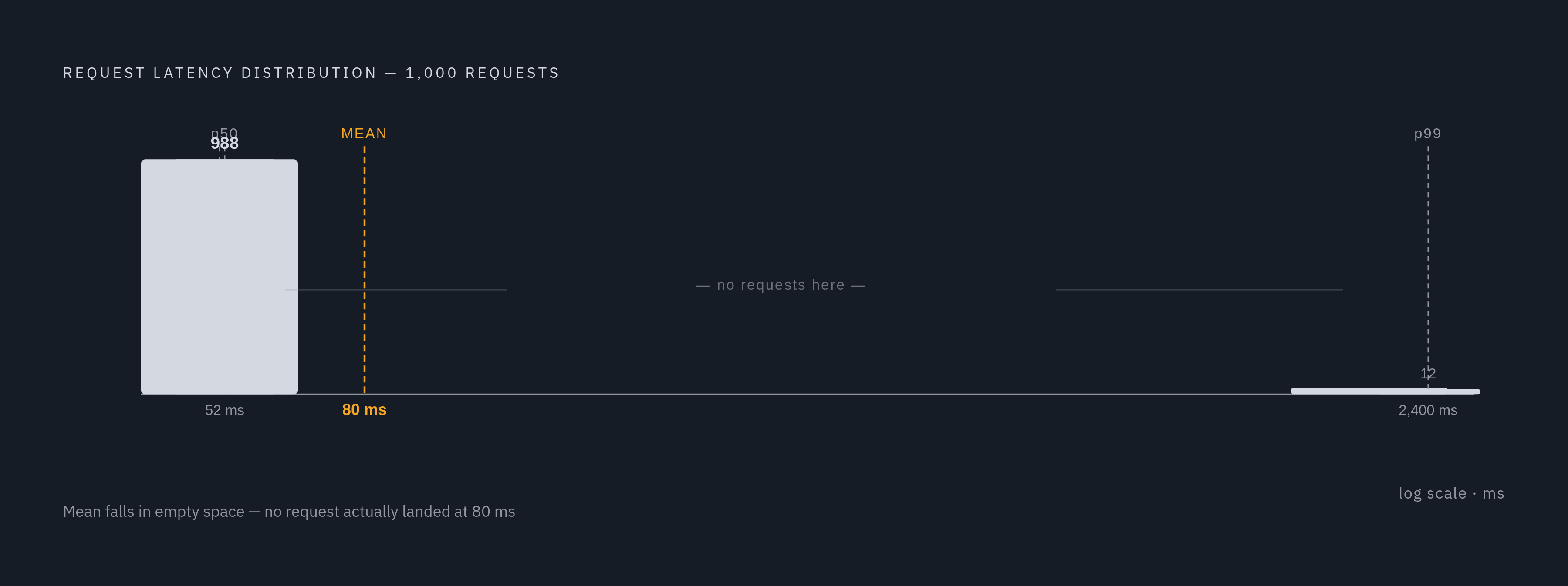
A worked example shows exactly how badly this goes wrong. Take 1,000 requests. 988 of them finish in 52 milliseconds. The remaining 12 stall out at 2,400 milliseconds. The mean comes out around 80 milliseconds. Sounds fine, right? But the p99, the actual worst 1% of requests, is 2,400 milliseconds, 30 times higher than the mean. That's 30 times higher than the mean.

So who experienced 80 milliseconds? Nobody. Not one request in that dataset landed anywhere near 80 milliseconds. The fast group ran at 52, the slow group ran at 2,400, and the average sits in a gap where no actual event occurred. It describes a request that never happened, while hiding the two groups that did.

Now scale it up. At one million requests, that "small" 1.2% tail becomes something like 12,000 slow requests. That's not a rounding error anymore, it's a user population. Twelve thousand people (or twelve thousand agent calls, or twelve thousand transactions) hitting a multi-second delay, sitting quietly behind a mean that still looks perfectly healthy on a dashboard. The average isn't lying exactly, but it's answering a question nobody asked while ignoring the one that matters.

What the standard percentile vocabulary covers

Percentiles solve the distortion averaging causes by pointing at a specific spot in the sorted distribution instead of blending everything together. The standard set used in production monitoring runs p50, p95, p99, and p99.9, and each one earns its place by answering a different question.

p50, the median, tells you what a typical request looks like. It's the number to watch for capacity planning and for catching regressions in the common path, the stuff that happens to almost everyone almost all the time.

p95 and p99 are where the tail starts to bite. This is what users at the edge of the distribution actually experience, and it's the range most user-facing service level objectives should target. If a system serves a million requests a day, the p99 is what a meaningful chunk of real sessions run into.

p99.9 and beyond matter when rare failures are still unacceptable failures. Financial transactions. Identity token issuance. Agentic tool calls, where a single slow step can stall an entire chain of automated reasoning. Nobody tolerates a 1-in-1,000 failure rate on a wire transfer just because it's statistically rare.

Each percentile is a real position in a real, sorted list of numbers. That property, being an exact marker in an ordered dataset, is precisely what makes them so easy to compute wrong once you start aggregating across machines. Which is where things get interesting.

Why averaging percentiles produces numbers that mean nothing

Percentiles are what statisticians call order statistics. Computing one means sorting the entire distribution and picking a position out of it. Once that's done, once a single p99 number has been produced, it can't be recombined with another p99 number to produce a correct answer. The information required to do that math correctly was thrown away the moment each node collapsed its full distribution down to one point.

But what if you just average the p99s across all your hosts? Seems reasonable. That reasoning fails, because averaging the p99s across all your hosts does not produce the true p99.

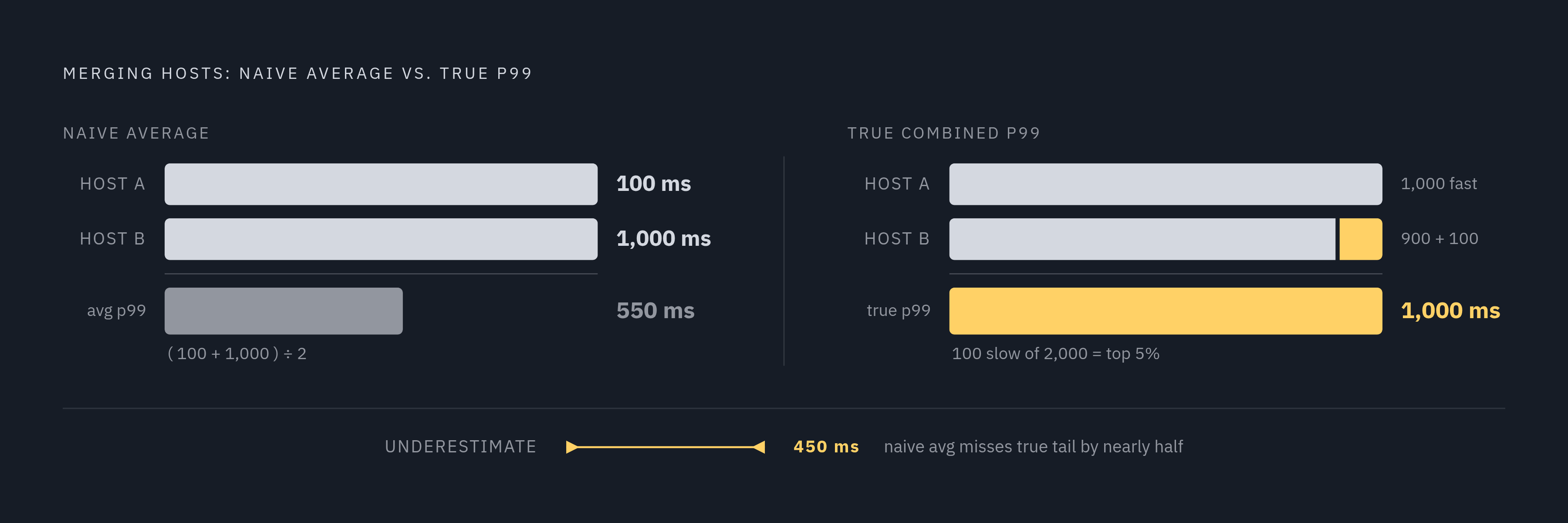
Take two hosts. Host A serves 1,000 requests, all of them landing at 100 milliseconds. Its p99 is 100 milliseconds. Host B serves 1,000 requests too, but 900 are at 100 milliseconds and 100 are at 1,000 milliseconds. Its p99 is 1,000 milliseconds. Average those two p99 values together and you get 550 milliseconds.

Now compute the actual p99 across all 2,000 requests combined. It's 1,000 milliseconds, because that latency covers the slowest cohort across the combined 2,000 requests. The naive average said 550. Reality said 1,000. The naive approach understated the true tail by nearly half, and weighting by request count doesn't rescue it, because the shape of each host's distribution is already gone by the time you're averaging.

The same failure occurs across time. Averaging 60 one-minute p99 values does not produce the correct hourly p99. It produces a number that resembles it, sometimes, by coincidence, and is wrong the rest of the time in ways that are hard to catch unless someone goes and checks the raw data.

How approximation algorithms make correct aggregation tractable at scale

Correct percentile math wants the full sorted list of every observation. At telemetry scale, that's not workable: storing every single latency measurement forever, across every host, isn't something most systems can afford. So the engineering answer is approximation with known, bounded error, using data structures built specifically to survive merging.

Two families dominate here.

Bucketed histograms (the kind found in Prometheus classic histograms and OpenTelemetry's explicit-bucket histograms) count how many observations fall into predefined ranges. They merge cleanly across hosts and time windows, because adding two histograms together is just adding bucket counts. Accuracy depends entirely on how well the bucket boundaries match the actual shape of the data.

Quantile sketches, HDR Histogram, t-digest, and DDSketch among them, adapt their internal structure to the data itself rather than relying on fixed buckets set in advance. They're mergeable too, but each one trades accuracy and mergeability differently.

HDR Histogram, built by Gil Tene, uses a fixed memory footprint and does no allocation during recording or iteration, which matters a lot when you're measuring latency inside a hot path and don't want the measurement itself to become a source of latency. It holds configurable precision across a wide dynamic range, commonly tuned to roughly plus or minus 1%, or tighter, around 0.1%. Recorded benchmarks put write performance at 3-significant-digit precision around 51 nanoseconds in Rust and 184 nanoseconds in Java, with p99 reads over roughly 20,000 populated counters landing near 49.1 microseconds in Rust and 54.7 microseconds in Java (measured on an EC2 t3.micro, 100,000 records, 7 runs, median of per-run p99s). HDR Histogram earns its keep when accuracy in the measurement space itself is the priority. Its weak spot is unbounded value ranges and merging across distributions with very different shapes.

t-digest, from Dunning and Ertl, takes a different approach: it clusters observations into centroids sized specifically to be more accurate at the extremes, which is exactly where percentile accuracy tends to matter most. The MergingDigest variant is the one to know about, since it balances accuracy, size, and speed well, with no dynamic allocation after it's built. Most insertions are fast, though compaction runs every few hundred to few thousand samples and costs more when it does, an amortized cost rather than a per-insert one. The trade t-digest makes against HDR Histogram is giving up a fixed relative-error profile in exchange for full mergeability, which is the property that matters most once data is scattered across a fleet.

Neither family is universally correct. The choice depends on whether the priority is fixed-precision accuracy or clean mergeability across a distributed system, and a benchmark report that can be trusted says which one it used.

Coordinated omission: the measurement error that hides the worst latency

None of the aggregation math above matters if the raw data going in is already broken. Gil Tene named this failure mode "coordinated omission" in his talk "How NOT to Measure Latency," and it survives every approximation algorithm mentioned above, because it corrupts the input before any algorithm ever touches it.

A load generator sends a request, waits for the response, then sends the next one. That's a closed-loop design, and it seems harmless until the server stalls. During that stall, the load generator isn't sending anything, because it's still waiting on the response that's stuck. The requests that would have arrived during that stall window? They're never sent. Never recorded. Never counted anywhere.

So the very requests that would have captured the worst behavior, the ones queued up behind a struggling server, simply don't exist in the dataset. The tail gets understated because the measurement approach was structurally blind to the failure it was supposed to catch.

At high throughput, this gets worse fast. A single stall event can suppress the latency of many in-flight requests at once, and the benchmark ends up looking cleanest exactly when the system was struggling hardest. That's the cruel irony of coordinated omission: it hides the problem in direct proportion to how bad the problem actually is.

What a complete latency benchmark report must include

Given all that, what does a trustworthy latency benchmark actually need to show its work?

At minimum, it reports p50, p95, and p99 as independently derived values, not blended or averaged across windows or hosts. A single percentile in isolation doesn't say much. A set of them, viewed together, shows whether the tail rises gradually or snaps upward sharply, which is often the more useful signal.

The report should also disclose its aggregation method: which algorithm did the work (bucketed histograms, t-digest, HDR Histogram, DDSketch), what precision or error bounds it operates under, and whether the published percentiles were re-derived from merged raw distributions or, worse, averaged after the fact.

And it needs to disclose its load model. Closed-loop or open-loop? Was coordinated-omission correction applied? What throughput was targeted, and what throughput was actually achieved? A benchmark that skips these details might still be honest, but there's no way for a reader to check.

How benchmark methodology choices show up in published results

Theory is one thing. Published numbers are where methodology either holds up or falls apart, and a few examples make the stakes concrete.

One vector database benchmark standardized on 1 million vectors at 1,536 dimensions, reporting single-query latency at p50 and p99, taking the median across three independent runs. The results: an open-source vector engine at 4 milliseconds p50 and 25 milliseconds p99, a managed vector service at 8 milliseconds p50 and 45 milliseconds p99, and a managed document database at 22 milliseconds p50 and 110 milliseconds p99. In each case, p99 lands meaningfully higher than the median. That ratio, not just the raw numbers, is the signal to read. It says something consistent about tail behavior across very different absolute latencies. Were those p99 values re-derived from the merged raw distributions across all three runs, or averaged from three separately computed p99s? "Median of three independent runs" should mean three separate p99 calculations, with the median taken across those three results, not an average of pre-computed percentiles. The methodology note doesn't spell that out explicitly, and it should.

A separate MySQL ecosystem benchmark took the opposite approach, reporting throughput in transactions per second rather than latency percentiles at all. That's a legitimate choice for capacity planning; a database engine's TPS ceiling tells an operator something real about hardware headroom. One engine led read-write workloads at 32 GB buffer pool size with roughly 13,385 and 13,325 TPS at 512 threads across two tested versions. Another dominated read-only workloads at 32,392 TPS at 128 threads, about 38% ahead of the next-best engine tested. An older release collapsed under concurrency: it peaked at 13,684 TPS read-only at 32 threads, then fell to 3,889 TPS at 512 threads. That collapse is a proxy for latency exploding under load, even though the benchmark never reports the p99 directly. Throughput and latency percentiles answer different questions, and reading one without the other leaves a real gap in the picture. A system can hold respectable TPS while its slowest 1% of transactions quietly balloon, and a throughput-only report cannot reveal that.

Service level agreements offer another angle on why p99 specifically recurs in practice. One cloud database SLA commits to a five-second recovery point objective and a 30-second recovery time objective, with service credits tied to any breach. That's not a benchmark claim, it's a commercial commitment, but it's telling that the binding language reaches for p99 rather than an average. Even in a contract, the tail is what gets guaranteed, because the tail is what customers actually notice.

Benchmarking guidance separates the client running the load test from the server being tested, putting each on its own machine. That's common practice, and it's disclosed as a trade-off, since it introduces real network round-trip time into the measured latency. Whether a benchmark ran client and server on the same box or split across machines connected by a network is part of the methodology. It changes the numbers.

Why tail latency has higher stakes for agentic and parallel query workloads

Everything above affects how often and how accurately software can decide on its own when to query and how often, as those decisions come to depend on it.

A human clicking through an app hits the p99 case rarely, maybe once in a long session, and probably shrugs it off. An agent issuing dozens of queries in rapid succession, in parallel, chained together so that each step depends on the last, runs into that same p99 case far more often, purely as a function of volume. One might argue that's just a math problem: more attempts means more chances to land in the tail. That's true, but it understates the consequence, because an agentic pipeline doesn't experience one slow request in isolation. It experiences a slow link in the middle of a chain, and everything downstream waits on it.

That raises an important question: what happens when the slow 1% isn't a rare inconvenience but a routine cost of doing business at agent scale? A workload that fires off many parallel queries per task, repeated throughout the day, samples the tail constantly, by construction. It's sampling it constantly, by construction. The benchmark numbers that looked like an edge case for a human user become a load-bearing part of the system's real-world performance for an automated one.

Which is exactly why p99 and p99.9, treated for years as numbers mostly for the ops team to squint at, deserve a wider audience now. Anyone building on top of a database that agents will query heavily is, whether they realize it or not, building on top of that tail.