Cost Predictability Risk in Consumption-Based OLAP Pricing

Consumption-based OLAP pricing takes financial volatility that used to sit on a vendor's income statement, and it moves that volatility onto the customer's operating budget. That transfer is a structural feature of the pricing model, not a flaw that better monitoring can fix. Inside Consulting's 2026 white paper describes the logic: vendors align revenue to the value a customer actually gets, usage growth turns into natural revenue expansion, and the volatility that used to belong to the vendor now belongs to the customer's budget line. This is not a fringe experiment. The number of software companies using consumption-based pricing more than doubled between 2015 and 2024, according to McKinsey research cited in the same paper, which makes this the dominant direction for the industry rather than a niche alternative.

The variance has a specific cause: the unit a vendor meters, whether that's bytes scanned, compute-seconds, or credits, is not the same thing as the business outcome a customer is actually trying to buy. A seat-based contract ties cost to headcount, and finance can count that on one hand. A consumption contract ties cost to behavior: how a query is written, how often a warehouse spins up, how a workflow is scheduled. When the billing unit and the business outcome decouple like this, you can no longer estimate the bill; you can only guess at it.

Three billing unit types

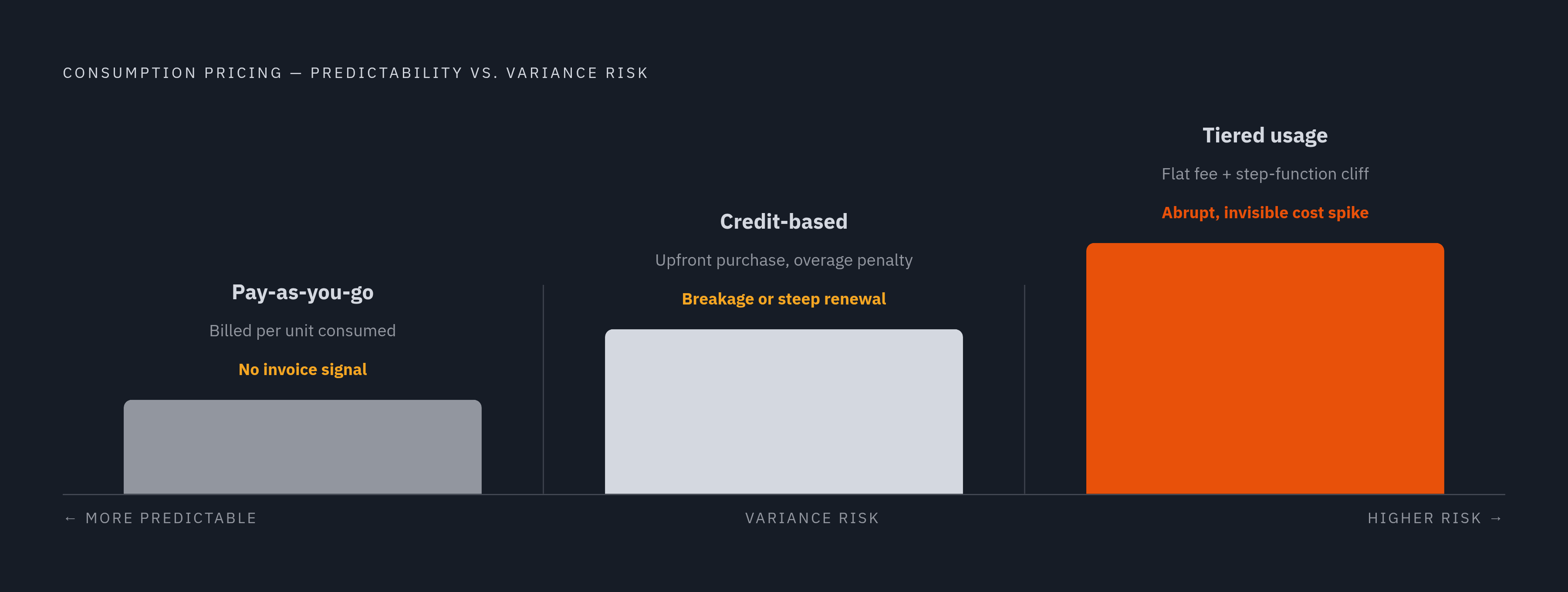
Before any forecast can be trusted, the meter itself needs scrutiny. The specific unit a vendor counts is the single most important variable in predicting what an OLAP bill will look like, and most buyers sign contracts without interrogating it closely enough. Consumption pricing comes in three broad flavors, and each one needs you to forecast it differently. Pay-as-you-go, or post-paid billing, charges exactly for what gets consumed and settles the bill at month-end. You get maximum flexibility and maximum variance, and you have no advance signal before the invoice lands. Credit-based pricing works the opposite way: the buyer purchases a bucket of credits upfront, the vendor benefits from breakage when credits go unused, and the buyer ends up choosing between waste or a forced early renewal at steep overage rates. Tiered usage splits the difference: a flat fee covers a baseline, but overage charges above it can hit a team as a step-function cliff with no warning.

CloudNuro's buyer's guide identifies the core trap: when pricing is based on multiple metrics at once, such as API calls, storage, and processing time, buyers struggle to estimate expenses because each dimension scales independently of the others. OLAP-specific meters make this worse rather than better. Compute credits, in the style Snowflake popularized, meter a combination of time and warehouse size. Bytes-scanned models, the kind BigQuery uses, meter the volume of data touched by a single query. Both are sensitive to the shape of a query in ways a seat count never was. A contract tied to credits or bytes scanned carries a second layer of risk beyond the pricing tier itself: credit-based deals that lack a negotiated rollover clause let unspent credits expire, and teams under end-of-term budget pressure often over-consume just to avoid losing value they already paid for.

How Snowflake-style compute credits amplify query-level variance

You see the abstract taxonomy turn concrete the moment you look at a single query or warehouse setting. In credit-based OLAP systems, one schema decision or one misconfigured warehouse can multiply the credit burn rate by an order of magnitude overnight, which makes the billing unit functionally unforecastable without governance applied at the level of individual queries. Peliqan's 2026 Snowflake analysis lays out the mechanism directly: compute makes up the large majority of the total bill, and a single oversized warehouse or a poorly written query running a full table scan can push credit burn up tenfold in a single night.

A second mechanism compounds the first, and it gets far less attention than it should. Most systems charge a minimum compute duration every time a warehouse starts up. If customer-facing OLAP serves thousands of concurrent users, every low-latency query event can trigger that minimum charge, so you can end up billed for far more compute than you actually used. So you need to see schema and query design as financial decisions as much as performance decisions. Denormalization, materialized views, and pre-aggregation set the ceiling on how much waste is possible, and the single anti-pattern that amplifies cost the most is running heavy OLAP queries without pre-aggregation, forcing a full scan on every request. The median Snowflake buyer pays $96,594 a year, and companies routinely report bills that run 200 to 300 percent above what they forecast. Snowflake has moved to address unpredictable billing directly: it launched simplified hybrid table pricing in March 2026 and uniform Snowpipe rates in December 2025, a sign that it recognizes the complaint. The structural mechanism causing those changes stays exactly where it was: compute-credit billing is still sensitive to how a query is shaped.

The secondary cost surface that S3-routed architectures add beneath the compute bill

Compute credits are only one layer of the bill. Many managed OLAP systems route every query through object storage, which opens a second billing surface that compute-focused pricing summaries don't show, and this surface can exceed the base storage cost by a wide margin. The sticker price for storage is rarely the issue. The real cost sits in the secondary and tertiary charges: PUT, COPY, POST, and LIST operations, GET requests, lifecycle transition fees, and egress charges, each arriving as its own separate line item. A 2025 analysis by CloudZero found that for data-intensive workloads, variable S3 costs can run three to five times higher than the base storage price.

The mechanics behind that multiple work like this: if a bucket has versioning enabled, its LIST calls get billed at the same rate as PUT and COPY operations, and a bucket holding many object versions can generate millions of LIST calls in a single month. Automated lifecycle transitions move objects between storage tiers to save money, but they charge a PUT request for every object moved, so transitioning millions of objects generates millions of billed PUT requests. Egress then sits on top of all of it as a multiplier: at meaningful data volumes with active monthly retrieval, storage plus egress alone can run into the thousands of dollars before a single compute credit gets counted.

The practical consequence appears on the wrong line item. When finance teams investigate unexplained S3 spend, they often trace it back to the OLAP routing layer rather than to S3 itself, so the cost lands on the wrong line, and you need an architectural fix rather than a contractual one. If an OLAP system separates compute from storage as a durability strategy, routing through object storage under the standard design is the cost of the architecture itself, not an avoidable side effect. So when you evaluate this risk, ask whether the hot-data path routes through S3 on every query, or whether a cache layer sits in front and absorbs that traffic first.

The gap between provisioned, actual, and billed usage

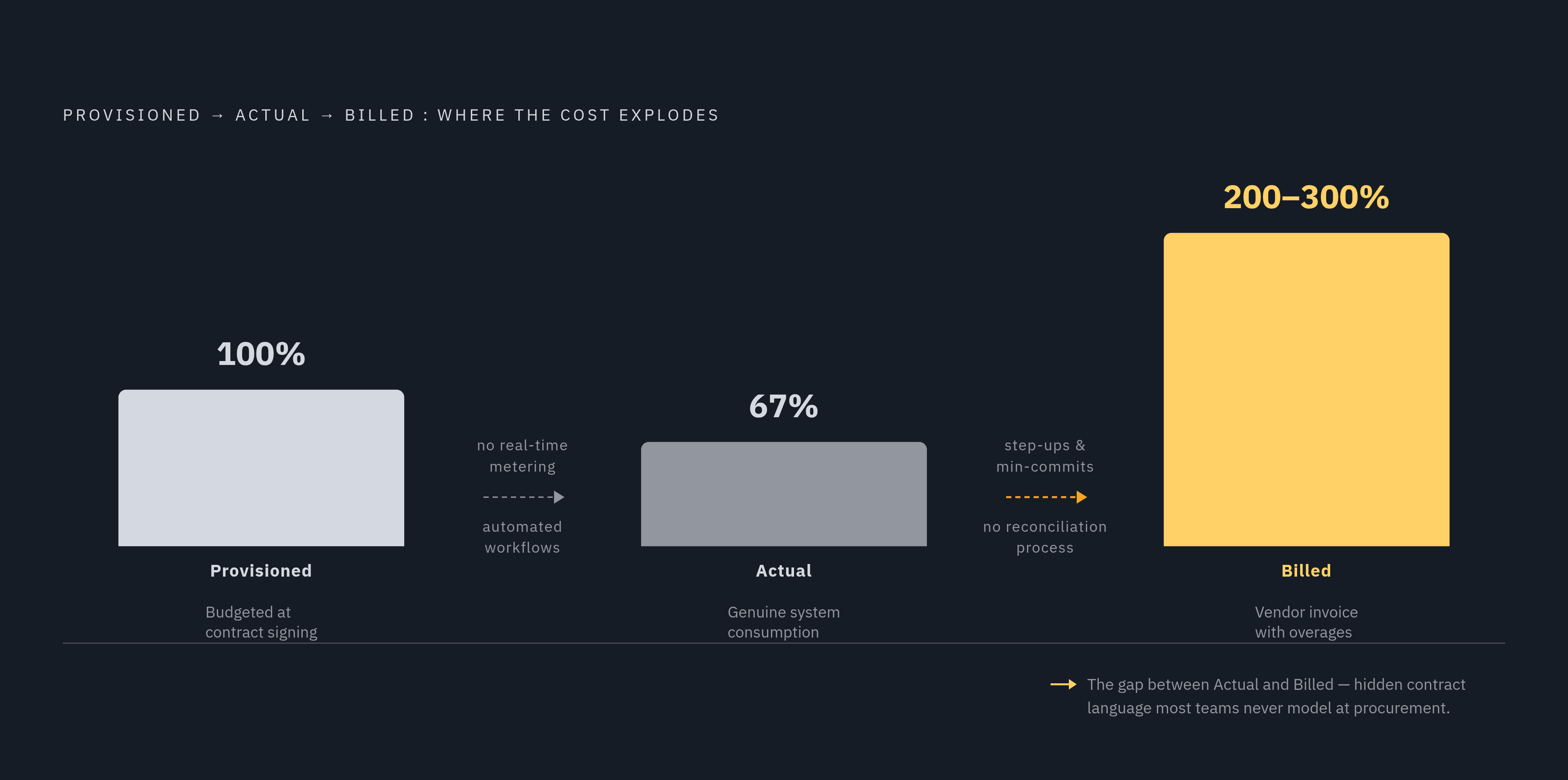
The mechanisms described so far explain where variance gets generated. The gap between what was budgeted, what was actually consumed, and what the vendor billed is the product of four compounding failure modes that most mid-market engineering teams have no systematic process to intercept.

Inside Consulting's 2026 white paper names the three numbers that organizations routinely fail to reconcile: provisioned usage, meaning what was budgeted or committed at contract signing; actual usage, meaning what the system genuinely consumed; and billed usage, meaning what the vendor invoiced, which often includes overages, minimum-commit true-ups, and usage-tier step-ups buried in contract language that nobody flagged during negotiation. Four failure modes drive the gap between those three numbers. There's no real-time metering visibility in most organizations, so finance learns the true cost only when the invoice lands rather than during the billing period itself. Contract language frequently embeds step-ups and minimum commits that were never modeled during procurement, so the cost structure baked into the agreement is a surprise even to the people who signed it. Most teams also lack any systematic reconciliation process between what the system reports as consumed and what the vendor actually invoices, leaving two separate records of truth that nobody is checking against each other. And consumption itself is driven by automated processes and workflows rather than by headcount, which makes the traditional per-seat mental model irrelevant to how the bill actually moves.

Under a seat-based model, cost holds steady if you don't hire anyone new. Large enterprises tend to absorb this risk better, because they run dedicated FinOps functions that watch consumption against contract terms in real time. Mid-market teams rarely have that function, so they tend to discover consumption variance after the fact, as a line on an invoice rather than a signal they caught early.

How agentic AI workloads break consumption forecasting

Every mechanism described above assumed a human was somewhere in the loop, deciding when to run a query or refresh a dashboard, and agentic AI, of which three main flavors exist, each with a different forecasting profile, removes that assumption. Agent access to OLAP systems is a different consumption pattern from human-driven query load: it defeats caching, it overwhelms existing cost models, and it produces billing spikes with no human decision behind them.

With human-driven workloads, an organization can hold a rough mental model of spend: how many analysts are active, when dashboards typically run, when the ETL job kicks off. Agents erase that model entirely, because they decide for themselves what steps to take, which tools to call, how often to retry a failed step, and how broadly to explore a dataset, all without asking permission first. A documented case makes the mechanism concrete. The OpenClaw GitHub issue #19534, filed in February 2026, describes a dynamic field in a system prompt, a "Current Date & Time" value, that changed on every single turn and defeated the cache completely. Cache reads dropped to zero and costs ran at a multiple of what the team expected. Any agent carrying a dynamic query parameter, whether that's a timestamp, a user ID, or a session token, will defeat OLAP query caching through the same mechanism and force a full re-scan on every call.

The scale of this shift is already visible in how AI budgets are allocated. Enterprise AI inference now makes up most of total AI spend, and agentic workflows burn far more tokens per task than a standard chatbot exchange, so agentic access is already the dominant AI cost driver, and agents probe OLAP harder than any other data layer. Right now, many teams make the forecasting mistake of treating an agent as if it were a human query source. An agent is a first-class database user with its own consumption profile, and any cost model built on human query patterns will miss what an agent actually does to a warehouse.

What PITR and recovery windows cost under consumption billing

A cost most teams haven't modeled appears when an active incident forces point-in-time recovery into use. Point-in-time recovery is now treated as a baseline requirement in enterprise OLAP contracts, but its cost structure under consumption billing, and its operational failure modes, rarely get modeled at the time a contract gets signed.

PITR forces a direct tradeoff under consumption pricing. Shorter retention windows cut storage spend, but they narrow how far back you can recover. Longer retention windows buy more flexibility, at the cost of storage charges that accumulate continuously and grow in step with transaction log volume. High-transaction OLAP databases can generate enormous log volume, and that volume adds meaningfully to total cost of ownership in a way that's typically absent from the pricing model a team evaluated at procurement, because it scales with write throughput rather than with raw data volume.

There's a hard ceiling on top of all of this that catches teams off guard. Cloud-native PITR comes with a fixed window limit: native point-in-time recovery in services like RDS, Aurora, and DynamoDB stops at 35 days. If a slow data-corruption bug, or a quiet deletion, is discovered weeks later, it can fall outside that window, and once the 35 days have passed, no recoverable history remains. That isn't a billing surprise in the way a compute spike is; it's a recovery-capability gap that a team only discovers once the thing it needed to recover is already gone, which makes it the one item on this list worth checking before an incident forces the question.