SLO Burn Rate Alerting in Streaming Ingest Environments
Adapt burn-rate alerting to streaming data by measuring delivery, not just broker health.

SLO burn-rate alerting in streaming ingest environments needs more than a new set of thresholds. It needs measurements that show whether all the data arrives on time, plus alert windows that tell ongoing loss apart from normal bursts. The underlying math still works, but its usefulness depends on adapting both the evidence it consumes and the decisions it triggers.
Why burn-rate alerting was designed for request/response services and what that assumption buys you
Threshold alerts often fire on spikes that end before anyone responds. Burn-rate alerting instead ties the signal to how quickly a service consumes its error budget. Google SRE Workbook chapter 5 develops this approach through progressively better alerting methods, judging them on precision, recall, detection time, and reset time. The aim is to detect reliability loss that warrants a response while leaving short-lived noise alone.
Burn rate is a unitless multiplier calculated by dividing the current error rate by the error budget rate. A burn rate of 1 means the service would use exactly its budget over the SLO compliance window if that pace continued. Higher multipliers shorten the time to exhaustion proportionally. Because the calculation uses an error ratio rather than a raw count, it puts failures in the context of traffic volume. The same number of errors can be serious for a low-traffic service and minor for a high-throughput one.
The dual-window design adds a test of persistence and recency. A long window establishes sustained impact, while a short window establishes that the problem is still current. Both must be above the threshold at the same time, so an old incident cannot keep an alert active through its long-window average alone. Elastic’s SLO burn-rate rule documentation makes the short window a fixed fraction of the long window. This pairing improves the balance between fast detection and precise paging that a single window struggles to achieve.
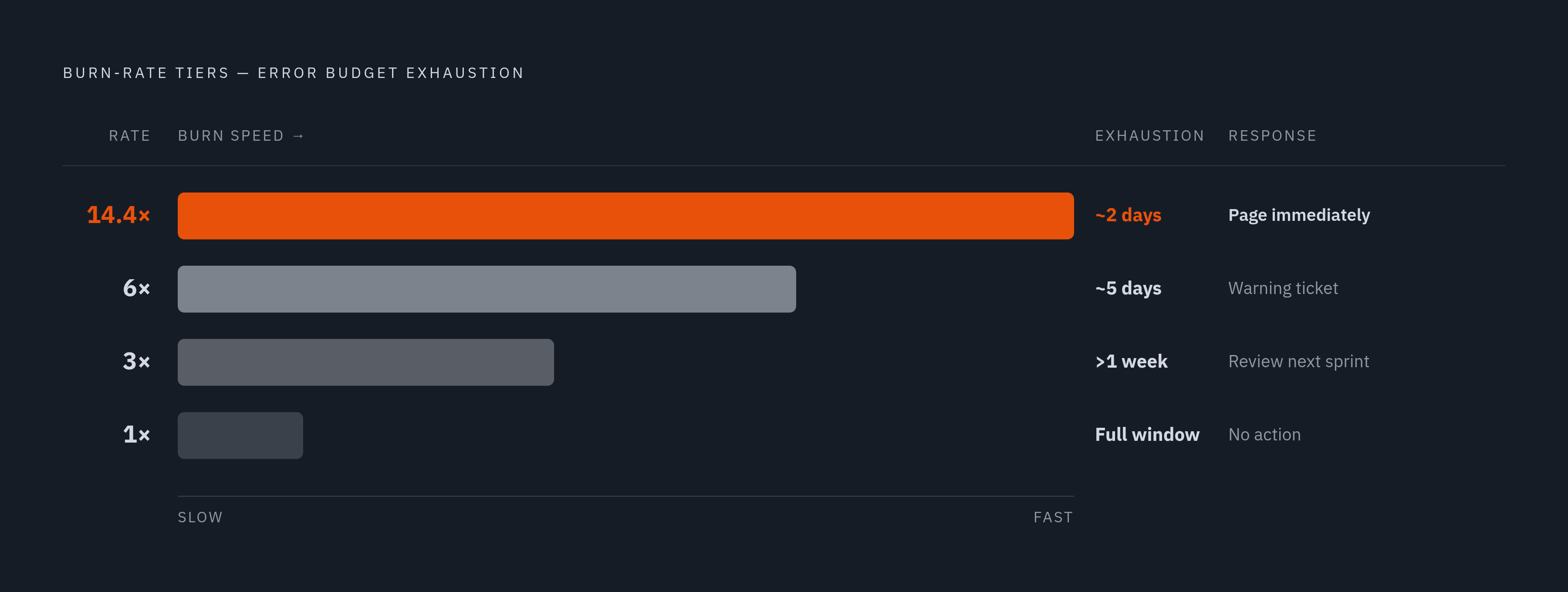
The canonical tiers translate burn speed into urgency. A 14.4× burn points to roughly two days until exhaustion and calls for an immediate critical page, while 6× points to roughly five days and a warning ticket. A 3× burn leaves more than a week and supports a slower response, while 1× is the sustainable pace. These horizons depend on the SLO window, with the threshold derived by dividing that window by the acceptable time to exhaustion. Underneath this framework sits a convenient assumption that bad events are request failures, countable one-to-one at a single measurement point.
The assumptions burn-rate alerting makes that streaming ingest violates
A message travels asynchronously through a producer, broker, stream processor, storage layer, and consumer. A failure at one hop may be invisible upstream and remain unnoticed until a consumer sees a gap or a flat line. So success at an early hop does not prove that the data product was delivered. Every part of the infrastructure can appear up while some telemetry never reaches durable storage.
A message may arrive late, a store may stop getting fresh rows, or some of the expected data may never arrive. Those are different failures for the downstream user, even when the broker accepts messages successfully. Broker CPU and topic lag cannot, by themselves, distinguish all these outcomes. The diagnostic gap is between the health of the machinery and the health of the data it delivers.
Traffic shape creates another mismatch. Device reporting intervals can produce smooth traffic, while a fleet restart can reconnect thousands of producers at once. A standard 5-minute short window can read that reconnect burst as a high error rate and help trigger a 14.4× alert that clears within minutes while using little of the budget. In that case, burst duration and error duration become confounded, and the window treats a normal workload pattern as evidence of an incident. Correcting the alert therefore requires changes to both what the SLI measures and how the windows interpret it.
What streaming ingest SLIs should actually measure
Completeness compares the messages that reach durable storage with the messages the producers sent. Freshness measures the maximum age of the latest committed row at the consumer side, while ingest latency measures the share of messages processed within a defined threshold at each pipeline stage. End-to-end latency measures the time from producer emission to consumer availability.
To use these measurements in burn-rate rules, each needs a definition of good and valid events. Message-based latency can use messages meeting the latency threshold as good events and total received messages as valid events. Freshness instead uses evaluation intervals, classifying them by whether maximum row age exceeds the freshness threshold. Each axis has its own SLO and error budget. This separation lets the end-to-end signal describe the user’s problem while the inner SLIs help localize the responsible hop.
Completeness is the hardest to count because the ingest layer cannot directly see everything a producer tried to send. Device-side sequence numbers show gaps, but they need support from the firmware and a way to handle counter resets on reboot. Broker-side accepted-message counters compared with storage writes are simpler, but miss losses before the broker. Synthetic probes test the full path with a canary producer emitting at a known rate, although they cover only that probe’s traffic pattern. The denominator therefore defines the measurement’s blind spot as well as its accuracy.
That choice also affects cardinality. Per-device labels multiplied by histogram buckets make the series count grow with fleet size even when meaningful reliability distinctions stay the same. Pre-aggregate error and total counts into tenant tiers and pipeline stages before burn-rate evaluation, and use entity groups for narrower slices. Even a correctly defined SLI falls short if standard dual-window rules mistake ingest bursts for ongoing budget loss.
How to set window lengths and thresholds when ingest traffic is bursty
The first tuning question concerns how long legitimate bursts last. Historical ingest traces can show the typical reconnect storm and the longest sustained legitimate burst. Those durations give a basis for choosing a short window and adjusting the 5 minutes to fit the workload. When producers reconnect and replay buffered messages, a window that mainly captures the replay can exaggerate its significance. Widening that window beyond the characteristic burst duration reduces this risk without simply raising the threshold and delaying detection of real burns.
Window length still works through an average that includes bursts. The short-window result must be considered together with the long-window result, and both must exceed the same threshold. The long window should span at least several burst cycles so it can distinguish sustained loss from closely spaced bursts. If a fleet restart stabilizes within a few minutes, a 1-hour long window is an example of a window that outlasts it while retaining sensitivity to problems that compound over hours. The appropriate pairing depends on the workload’s burst profile.
Elastic’s fixed short-to-long-window ratio constrains this choice in its implementation. Raw Prometheus rules allow teams to depart from that ratio when the workload justifies it. The standard 14.4× and 6× thresholds remain starting points, but threshold changes should reflect the intended budget-exhaustion horizon. A Prometheus for clause can add an evaluation-jitter buffer after both window conditions become true. That buffer complements the window design rather than replacing the need to understand burst duration.
Time is not the only source of dilution. A fleet-wide completeness SLI can remain above target while a subset of partitions loses all its messages, because the healthy majority dominates the denominator. Compute burn rates for partition groups, grouped by region, tenant tier, or pipeline stage, as well as for the fleet. Use the group-level signal for the critical tier and the fleet-wide signal for lower tiers. This preserves visibility into localized freshness or completeness failures without requiring an SLI for every device.
When valid events approach zero, one dropped message can yield a burn rate above 14.4× without providing stable evidence for a page. Google SRE Workbook chapter 5 identifies low traffic as a precision hazard, and the same hazard appears within sparse ingest partitions. Available mitigations include suppressing ratio-based alerts below a minimum event count, lengthening the evaluation window for low-traffic groups, or using synthetic canaries instead.
Implementing multi-window burn-rate rules for ingest SLIs in Prometheus
Prometheus recording rules keep the familiar burn-rate structure, but use what happens to the ingested data as their inputs. For a completeness measurement based on received messages, derive the error ratio from dropped-message counters divided by received-message counters, summed by pipeline stage and tenant tier. That denominator limits the claim to the received population, leaving producer attempts outside that population unmeasured. Use the chosen SLO target to create a burn-rate series for each evaluation window. Computing these series ahead of time keeps alert evaluation from having to use raw, high-cardinality counters.
Freshness needs a different input, though its alerts have a similar structure. Its error ratio is the proportion of evaluation intervals in which maximum row age exceeds the freshness threshold. Recording rules must align those intervals and lookback windows carefully because a stale store can persist across many scrapes. Repeated stale observations represent time spent outside the freshness objective.
The alert rules have separate completeness and freshness families, with IngestCompletenessHighBurn using a 1-hour long-window burn above 14.4× for a critical page alongside the short-window condition adjusted for the workload, and IngestCompletenessMidBurn using a 6-hour long window above 6× for a warning ticket alongside its short window. In each case, Prometheus uses and to pair matching long- and short-window recording series that are above the same threshold. The critical expression uses the partition-group granularity established earlier, with any minimum-event guard and evaluation buffer applied to that rule.
Freshness alerts follow their own tier structure using the stale-interval recordings. Completeness and freshness should not collapse into one composite SLI, because their separate signals are needed to identify the failing part of the pipeline. Both families also need a companion absence alert on the SLI series, using absent() or its equivalent. A failed scrape target, crashed exporter, or relabeling rule that drops a series can otherwise leave the burn alert without data to evaluate. This meta-alert is especially important when the exporter is colocated with the pipeline, since one incident can disable both delivery and its measurement.
Using error budget policy to govern how teams respond to ingest burn alerts
A burn alert needs a pre-agreed mandate. At 14.4×, the response is to halt deployments and mitigate immediately, including pipeline configuration changes such as schema changes or partition rebalancing. At 6×, the policy calls for an incident ticket with a defined resolution window, while 3× calls for dashboard tracking and review in the next sprint. At 1×, no action is required.
Ownership must follow the SLI decomposition. The team responsible for broker configuration owns completeness burn alerts, while the storage-layer team owns freshness burn alerts. After an acknowledged critical alert, the on-call engineer can calculate how much of the monthly budget the incident consumed. Tracking consumption separately for each SLI axis then distinguishes recurring completeness loss from a one-time freshness spike and gives reliability work a quantitative basis. Burn-rate alerting becomes useful for streaming ingest when its budgets describe the data users receive, its windows reflect how that data moves, and its policy assigns responsibility for restoring it.