Kafka Connect Consumer Configuration for High-Throughput Pipelines

High throughput in Kafka Connect depends on configuration choices that work together. Consumer fetch sizing, task parallelism, and worker resources decide whether a sink keeps up or falls behind. The way to tune them is to start with the pipeline’s structural limits, then size batches around what the destination can write and what the system can safely replay after failure.

How Kafka Connect moves data and where throughput is actually decided

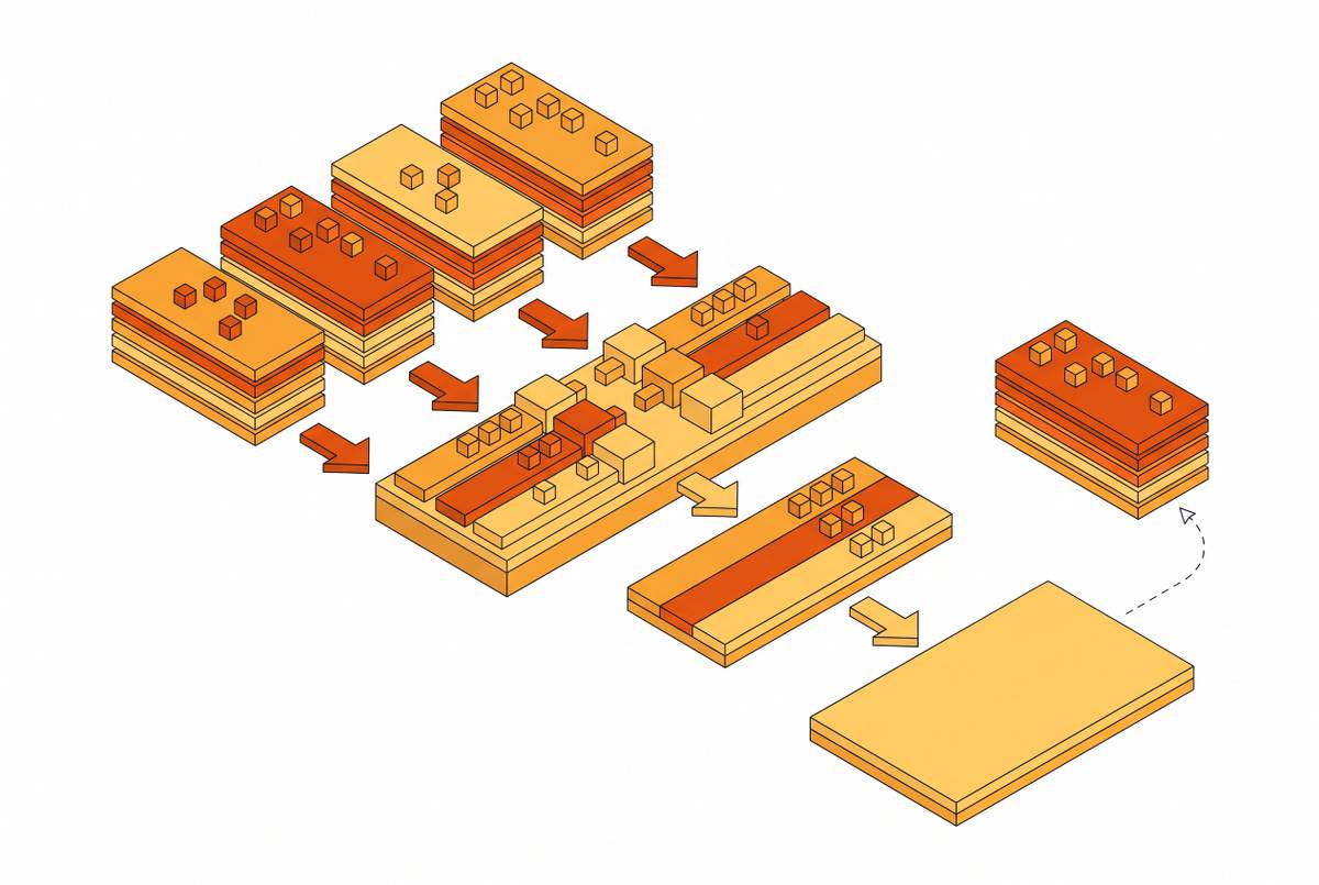
Kafka Connect divides the work among workers, connectors, and tasks. Workers are runtime processes, connectors define the copy logic, and tasks perform the reads or writes across worker nodes. Red Hat Streams documentation diagrams the sink path from a source Kafka topic through Connect tasks, a sink message queue, and a consumer buffer to the external destination. The runtime’s consumers retrieve messages from Kafka.

Configuration acts at three points in this path. It controls how much data arrives per fetch, how many tasks can work in parallel, and what resources the workers have available. These limits depend on one another. A partition is processed sequentially within one task, so task count cannot create parallel work beyond the partition topology. Broker and network capacity alone therefore do not determine the throughput a connector achieves.

Why fetch sizing is the first dial to turn for sink connector throughput

For a sink connector, fetch sizing sets how much data arrives in each broker round-trip. Undersized fetches leave capacity unused even when several tasks are running. Three settings define the volume. fetch.min.bytes sets the minimum data the broker tries to accumulate before responding, while fetch.max.bytes limits the total fetch response across partitions. Within that response, max.partition.fetch.bytes caps how much data can come from each partition.

The broker also needs a wait budget. fetch.max.wait.ms controls how long it holds a request open while trying to satisfy fetch.min.bytes. Raising the minimum and allowing more time can produce fuller batches, but the wait adds latency when data does not arrive quickly enough. How much waiting can the workload accept? A latency-sensitive path and a batch-oriented analytical pipeline need not make the same trade-off.

A high-throughput starting point is fetch.min.bytes=65536 (64 KB), fetch.max.wait.ms=500, max.partition.fetch.bytes=10485760 (10 MB), and fetch.max.bytes=104857600 (100 MB). These are reference values. The right combination depends on message sizes and destination write latency. The total and per-partition limits also need to agree, because a restrictive total response budget can undermine a larger per-partition allowance.

What max.poll.records actually controls and the rebalance risk of getting it wrong

Fetch volume is not the same as the batch a task receives from a poll. max.poll.records controls that visible record count. A smaller value keeps the pending batch smaller but means more polls and more overhead from polling. Larger values can improve batch-oriented throughput. They also widen the window of uncommitted records.

When a task restarts or a new task joins, a rebalancing task may need to finish its pending poll batch before it can commit offsets, so other tasks have to wait. If sink writes are slow, a large batch prolongs that wait and can turn a rebalance into a cascade of delayed work. Bigger is not automatically better.

The replay window depends on how many uncommitted records each task has, the batch size, and the commit interval. Raising max.poll.records expands that exposure directly, so batch-oriented connectors can justify a higher value only in relation to sink write latency. Paths that are sensitive to latency benefit from less time between commits. Keeping offsets safe also requires enable.auto.commit=false, so the framework controls commits around sink writes. Throughput gained by enlarging batches must therefore be weighed against the duplicate work possible after interruption.

How tasks.max and partition count set the parallelism ceiling — and how to hit it

Task parallelism offers a different way to increase throughput without continually enlarging each task’s pending batch. More tasks can divide the work, but only while partitions are available and the destination can absorb concurrent writes. For S3 sink connectors consuming CDC events, the target is one task per consumed Kafka partition, with tasks.max matching that count. Setting it higher adds no useful parallelism and wastes worker resources.

For relational sinks, database capacity is a co-constraint. Aggressive task scaling can exhaust connections or increase lock contention, so tasks.max needs to be planned with the connection pool and max_connections. A JDBC sink reference starts with max.poll.records=500 and a batch.size matched to RDBMS write capacity. Conservative values for errors.retry.timeout and errors.retry.delay.max.ms belong in that same plan. Consumer capacity is not the destination’s write budget.

Adding workers helps when workers run out of CPU or memory, or when tasks are spread unevenly across them. It does not repair too few partitions, destination throttling, or broker storage saturation. Red Hat’s documentation recommends first providing enough CPU and memory, then adding parallel tasks through tasksMax and worker nodes through replicas. Its approach is iterative. Each increase in deployment size needs to improve throughput as planned.

CDC source connectors break the parallelism model and require a different approach

The task-scaling model breaks for an important class of CDC sources. On Confluent Cloud, MySQL CDC Source and MongoDB CDC Source each permit only one task per connector. Raising tasks.max cannot make them execute several tasks. Horizontal scaling instead requires multiple connector instances against separate source shards. A reader expecting these connectors to scale like a standard JDBC source would otherwise tune a setting that cannot help.

This restriction is not universal across CDC. Google Cloud Spanner CDC Source and Oracle CDC Source support multiple tasks, so how a connector works sets how it can scale. Long-running snapshots create a separate coordination concern because worker rebalances historically forced interrupted snapshots to restart. Confluent described internal checks and metrics to protect tasks doing snapshots or other long-running transactions from interruption. It scheduled the enhancement across Debezium-based CDC connectors by the end of Q4 2025, with MongoDB connector support following in Q1 2026.

Source connector producer settings that determine what the sink has to handle

The sink’s workload begins upstream, where producer settings shape the batches it must absorb. Poor batching, uncompressed data, and oversized individual messages cannot be fully offset by sink fetch tuning. Red Hat’s documentation places source producer batch.size and linger.ms settings under the producer.override.* prefix. producer.override.buffer.memory sets the total bytes available for producer buffering.

The source’s batch.size should reflect the number of records the connector returns multiplied by their average size. Its default of 16 KB is too small for most high-throughput sources. A short linger.ms gives the producer time to accumulate records, reducing per-message overhead. Batching and compression reinforce each other by reducing network bandwidth and broker disk I/O. That upstream efficiency changes the conditions under which sink-side fetch and poll sizes are chosen.

Serialization shapes those conditions too. JSON’s verbose encoding creates larger messages and higher per-record overhead, while Avro or Protobuf with a Schema Registry provides smaller messages, schema validation, and schema evolution. The recommendation for high-throughput paths is to use those binary formats. Once the stream’s encoding, batching, and compression change, max.partition.fetch.bytes and max.poll.records need to fit the new message sizes and the cost of writing them to the sink. A record count alone does not describe the work in a batch.

Worker-level settings that bound all connector-level tuning

Correct connector settings can still underperform when workers lack headroom or coordination topics are poorly provisioned. Pre-create internal topics with the correct replication and compaction settings as a practical starting point. Offset flushing is another shared constraint. offset.flush.timeout.ms controls how long workers wait for in-flight messages to be acknowledged before flushing offsets. Red Hat’s documentation recommends increasing it when the source queue of outstanding messages grows unmanageable, so high load does not cause premature flush failures.

If a source producer cannot keep up, buffering blocks until max.block.ms expires, with new messages unable to enter until unacknowledged messages are flushed. More buffering is not unlimited relief. Complex or numerous Single Message Transforms also add CPU work for every record, so complex transformations should move from connectors to Kafka Streams. Worker sizing must accommodate that remaining work. A production reference uses three worker replicas with memory limits of 4 Gi and substantial CPU allocation per worker, which provides a workload-specific sizing reference.

Backpressure, sink-side write semantics, and why throughput planning is a failure-mode exercise

Switching from a community connector that issued individual HTTP requests to the official connector using Elasticsearch’s bulk API produced roughly three times the throughput. No fetch parameter change achieved that result. The distinction went beyond how quickly the connector read from Kafka to how it wrote the data. A tuning plan that overlooks write semantics can optimize the wrong side of the bottleneck.

What happens when that destination slows down? Backpressure appears when a sink consumes faster than the destination can absorb its writes, and Kafka does not provide built-in cross-network backpressure mechanisms. The pressure is visible in growing consumer lag, timeout errors, or exhausted buffers. Settings for steady-state work must therefore also allow for sink throttling, task failures, and rebalances. The earlier choices about batches and parallelism set how much unfinished work is left when those events happen.

Recovery settings need to reflect those conditions before production. errors.tolerance=all with a dead letter queue allows continued processing under partial sink failures, while errors.retry.timeout and errors.retry.delay.max.ms should be reviewed and set to match sink recovery time. Setting errors.deadletterqueue.context.headers.enable=true preserves failure context for downstream inspection. Recovery also includes duplicate writes. Sink connectors should be planned around at-least-once delivery, because retries and rebalances can write a record again, making idempotent destination writes safer than an assumption of end-to-end exactly-once delivery.

Assembling the configuration decisions into a coherent tuning sequence

First, establish partition count and align tasks.max for standard connectors within the destination’s connection capacity. For single-task CDC sources, the plan instead needs to spread the work across source shards. Then raise fetch.min.bytes, fetch.max.bytes, and max.partition.fetch.bytes together, with fetch.max.wait.ms set around acceptable latency. Fetch tuning is the first consumer dial, but topology determines the space in which it can work.

Next, choose max.poll.records from sink write latency and the acceptable replay window. An analytical workload may favor fuller batches, but its destination still needs to complete them within a workable recovery budget. Source alignment follows. Review batch.size, linger.ms, and compression.type at the source connector level, and replace JSON with Avro or Protobuf for the high-throughput path.

Finally, provide worker capacity and coordination hygiene, including pre-created internal topics, an appropriate offset flush timeout under sustained load, and an audit of SMT complexity. Error tolerance, retries, and the dead letter queue belong before production. The final test is a failure-mode question. Can the chosen configuration handle a slower sink or an interrupted task without making its throughput gains come at the cost of too much replay work?